
Is a classic monetarist inflation theory established over 500 years ago, that states increases in the price level are solely determined by increases in the money supply. This theory is the core of monetarism.
The theory's prediction can be best shown via the Fisher Equation. This equation is an adaption of the equation of exchange and is named after the American economist Irving Fisher.
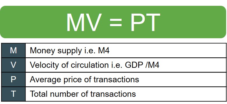
Now there are a few assumptions that monetarists impose on the equation in order for the theory and the subsequent results to hold. The most important of these assumptions is that T and V are always assumed to be constant values in the short-run at least. Monetarists particularly stress V is held constant because the demand for money is a function of income and this does not immediately change in the short-run from a change in M. Based on this assumption the equation cancels down to:

However, this assumption of a constant velocity of circulation in particular is often a sticking point for opposing Keynesian economists. This is because they argue that V must change even in the short-run because it is determined by human spending impulses from consumers and firms, which to assume is constant is illogical in their eyes. For instance, if the money supply is increased then the base rate must be changed and by doing so this affects economic agents demand for money (liquidity preferences).
If we take the monetarist assumptions as given and we get the simplified equation of M=P, any permanent change in the money supply creates an equal permanent change in the price level i.e. if the money supply doubles then the price level will double.
The mechanism of this inflation theory can be represented with the following graphs below:
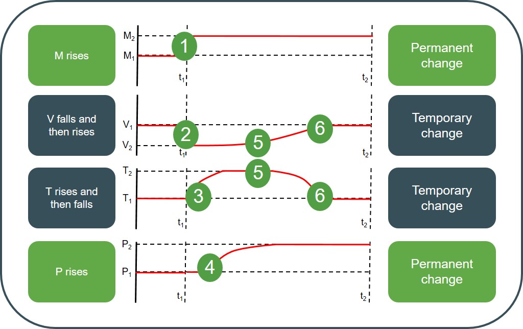
At period t1 the initial increase in the money supply causes the amount of money circulating in the economy to permanently increase from M1 to M2. This immediately causes the velocity of circulation to fall by an equal factor (V1 to V2) temporarily as each unit of currency does not change hands as many times within a year now there is more money circulating around. However, as the extra money begins to be spent by consumers the number of transactions (T) in the economy starts to gradually rise over time and this creates pressure for price level to rise over time (P) as a result of demand-pull inflation. As a result of more transactions being conducted in the economy, this starts to cause the velocity of circulation to rise over time as consumers make more transactions. But, as the price level rises this causes the number of transactions to fall back to its original level, which also means V also falls back to its original level, as consumer real incomes start to fall back to their original levels. So at the final equilibrium there is a higher price level with the same values for V and T.
The results of this theory can be represented in an AD/AS framework:
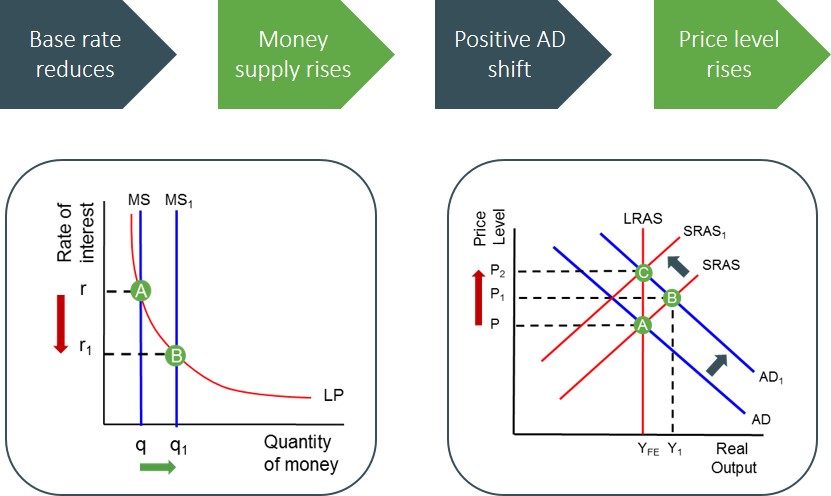
Assuming no accompanying LRAS curve shift is created this creates demand pull inflation and this can lead to an inflationary spiral, which is not always a problem for the economy, as this type of inflation arises from higher consumption, economic activity and results in growth. But, it is important to note that if the inflation rate becomes too high and volatile it becomes unhelpful as it undermines confidence and competitiveness in the long-run.
When evaluating the Quantity Theory of Money it is important to consider the following points:
- Accompanying Productivity Changes e.g. An outwards LRAS curve shift will create dis inflationary growth and will cause the predictions of the model to break down.
- Confidence Levels e.g. The theory assumes that consumers will always spend idle cash balances but they may prefer to hold onto cash balances.
- Level of Spare Capacity e.g. AD expansion may be absorbed and not create inflation if the economy is operating below the full employment level.
- Reverse Causation e.g. Money supply may accompany inflation rather than cause it.