Economic Terms

Is a pricing strategy, where products are sold by the firm at a price which is lower than the average cost of production or at a price low enough to make in unprofitable for other players to enter the market.

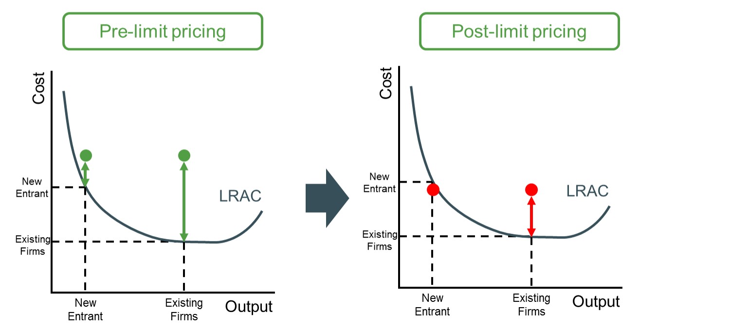
Below is a diagram to illustrate how this type of pricing strategy works. The reason why firms undertake this pricing strategy is to protect their market share and position by successfully deterring new entrants from coming into the market. To do this however the incumbent firm has to sacrifice the amount of supernormal profit they can achieve. In the lefthand side diagram the incumbent has lower costs than new entrants, therefore if they both charge the same price incumbent firms make a large amount of supernormal profit equal to the size of the green arrow. However, new entrants at that price can also make profits due to the price being positioned above their respective LRAC curve (but these profits are substantially lower). So if the incumbent firm did not change the pricing stratey new entrants would always have the profit incentive to enter the market. However, if the incumbent firm takes advantage of their lower costs and charges lower prices to a point which is equal to the point on the LRAC curve for new entrants. These entrants would no longer have any profit incentive to enter the market as they will be charging a price at the marginal cost and just making normal profit. Therefore, incumbent firms sacrifice short-term supernormal profits to guarantee larger long-term profits equal to the size of the red arrow in the right hand side diagram. This is an example of successful limit pricing with the aim to protect and consolidate their market share and position.

How easy it is to convert an asset into cash without experiencing a significant price impact or encashment delay e.g. an instant access deposit would be regarded as highly liquid while a property asset would be regarded as highly illiquid.

 

A ratio used to ensure that financial institutions have the necessary assets on hand to meet short-term liquidity requirements. Under this standard, the banks must hold a stock of unencumbered liquid assets to cover the total net cash outflows.

Below is the formula for calculating the LCR ratio. This ratio must exceed 1 in order for the financial institution to have enough liquid assets to cover volatile liabilites and remain in a solvent position on the balance sheet.

 

Is when a bank's balance sheet is in a position of a large liquidity mismatch. This can occur because of the liabilities maturing earlier than the assets and therefore bank's are left with no option but to sell their assets off at a firesale price prompting fears of a bank run and ultimately, if severe enough, can lead to bankruptcy.

Below is the logical sequence of reasoning for a liquidity crisis to summarise the main stages at which it occurs inside a bank's balance sheet.

Is a term associated with John Maynard Keynes defining situations where injections of new money into the banking system (e.g. quantitative easing) fail to stimulate lower interest rates and economic growth because economic agents hoard the extra cash and don’t spend it.

When a bank channels funds from savers to borrowers. The borrowers are deficit units - total expenditure exceeds total income - and require borrowed money from the bank to meet their spending plans. The loan requires borrowers to contractually pay back periodic payments linked with a specific interest rate to help banks make profit.

Below is the flowchart to illustrate how money flows from savers through the bank to borrowers.

The total productive capacity of an economy. It is equal to the full employment level of real output and is vertical at the point of full employment.

The LRAS curve illustrates that in the long-run unless there is a change in the size or productivity of the factors of production employed, supply will always exist at the full employment level and will not vary with price, as the economy is at full capacity. The diagram below highlights the typical shape of an LRAS curve.

 

When all factors of production are flexible i.e. the business is able to change capital and land when they wish to do so.

This curve is a straight vertical curve and shows that no matter the rate of inflation, in the long-run the rate of unemployment is consistently the same. In other words, in the long-run there is no trade-off between inflation and unemployment

Below is a diagram to show how the long-run version of the Phillips curve is formed. An expansion in AD creates economic growth and reduces unemployment below the natural rate of unemployment and this moves the economy to point B as jobs are created in the short-term. However workers now have more bargaining power, workers demand higher wages and this forces production costs up to a new higher level for firms, these then eventually get passed on as higher prices. Eventually in real terms nothing changes as the economy ends up at the natural rate of unemployment but just with a higher level of inflation. This is shown by the upwards shift of the short-run Phillips curve. This process continues to repeat itself with the only substantial effects being inflationary effects. Therefore the LRPC is derived from the continual shift up in the SRPC due to economic agents rational expectations.

 

 

 

The long term direction of output growth assumed to represent the productive potential of an economy.