Economic Terms

Is a market structure that describes the conditions required for intense competition to take place amongst firms in an market. This market structure is a contrast to a monopoly market. 

The assumptions that are required for perfect competition to hold are as follows:

1. Large number of buyers and sellers in the market.
2. No individual firm has significant market power to influence the market price - this outcome means that all firms are price takers and have to sell at the prevailing market price.
3. All firms sell a homogeneous products - the products that firms are selling are identical in terms of their product characteristics. This creates a horizontal (perfectly elastic) demand curve as all products that firms produce and sell are perfect substitutes for each other.
4. Freedom of firms to enter and exit a market - any firm can enter the market to enjoy profits as there are no barriers of entry present. However, firms can also freely leave the market costlessly if they are making a loss due to no barriers to exit being present. It is this assumption of freedom of entry and exit which means firms in this type of market structure will always make normal profits in the long-run.
5. Perfect knowledge available to all firms - sellers have perfect knowledge regarding their competitors and possible technological improvements available to the market and consumers have perfect knowledge of all firms prices and therefore will never buy the good at a higher price than at the market price. This assumption reinforces the prevailing market price that all firms must 'take'.   
6. Perfect mobility of factors of production - factors (e.g. labour and capital) can move from one production process to another to help complete different types of work. 

If firms operate in a market where all of these conditions are met it creates an environment of perfect competition. However, perfect competition is often discussed as being just a theoretical model of competition as a result of the unrealistic assumptions that are required to hold e.g. can a market ever have a situation of perfect knowledge across all firms and consumers?

Therefore, despite having a minimal role in terms of practical application, this model of competition is used as a comparison tool against other and more inefficient market structures such as a monopoly or oligopoly. This is because perfect competition leads to an efficient outcome in the long run in which social welfare is maximised, due to firms producing at the point that is allocatively and productively efficient. Therefore, the theory of perfect competition is a good evaluative tool in itself to use as a benchmark to assess the market outcomes from other types of market structure. 

A perfectly competitive firms demand curve is perfectly elastic (horizontal) at the prevailing market price, this means two things. First of all the firm can sell as a high quantity of the product they are producing as they want, without impacting the market price. But, the firm has to sell the quantity at the market price otherwise the demand for their product drops to zero. This is because consumers have perfect knowledge about other alternative sellers prices and will always buy the same product from the cheapest possible location. 

However, when graphically representing the perfect competition market structure for individual firms and the market in general it is important to consider the time horizon that firms are operating in. This is because the efficient outcome of perfect competition is only guaranteed in the long-run. In the short-run, firms produce at the profit maximisation point (P=MC), which can either be above, below or equal to the average cost of production. This means that firms can be making supernormal profit, normal profit or an economic loss in the short-run.

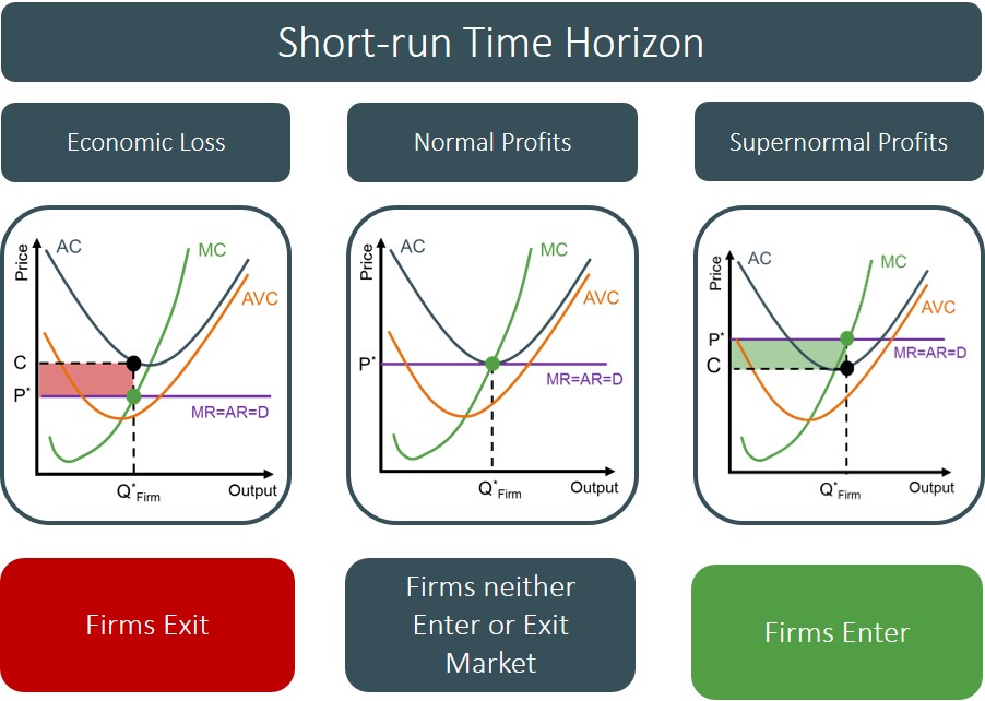
Whether a firm makes a profit or not in the short-run all depends on the type of market that the firm is operating in, the position of the firms average cost curve and the market price that prevails.

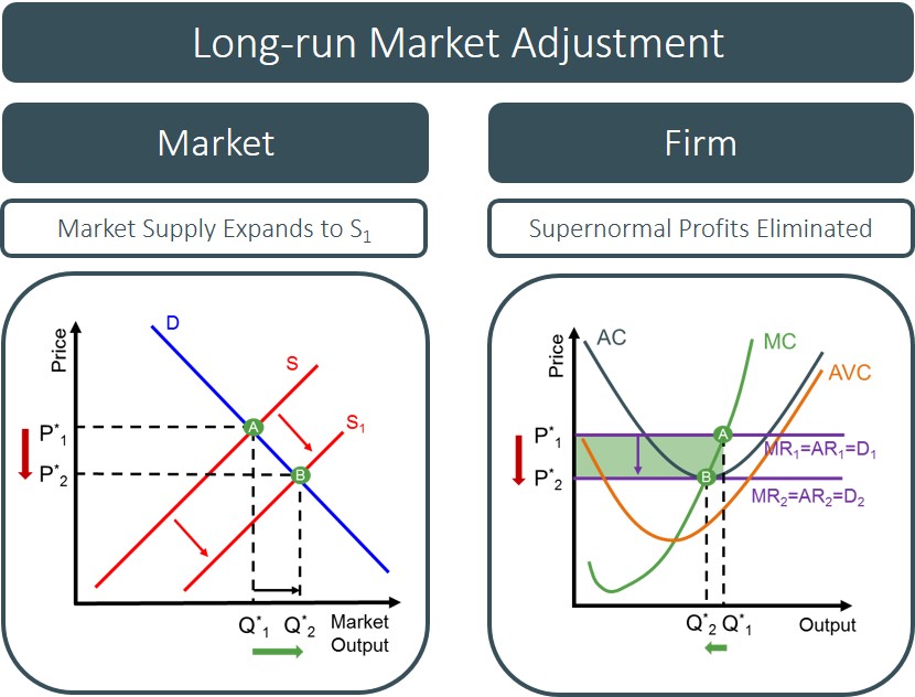
However, in the long-run all firms operating in a perfectly competitive market will make normal profits because of the fact that firms can freely enter and exit the market. For instance, if firms are making a profit in the short-run then this triggers firms that are not currently producing in the market to enter as the presence of supernormal profits lures and incentivises them to start producing. However, the decision for firms to enter increases the supply of goods produced in that market and without an accompanying equal change in demand, this creates excess supply in the market. The excess supply causes the price of the good to fall and as the price determines the position of the perfectly elastic demand curve firms face, this causes the profit maximisation point to fall closer to the average cost of production (which are assumed unchanged). This process of moving down a firms marginal revenue curve causes the amount of profits accruing to each firm to fall. Firms keep entering the market until eventually all supernormal profits have been eliminated and all firms are producing at the minimum of the average cost curve, signalling normal profits. This means all transactions will take place at the market equilibrium price and total output/consumption will be at the market equilibrium level. Below is an example of this market adjustment:

This process works in reverse if in the short-run firms were making an economic loss - firms are incentivised to leave to minimise their losses. In the case of normal profits being made in the short-run no change is made to the market.

This means the result of all firms in the long-run under perfect competition are shown below:

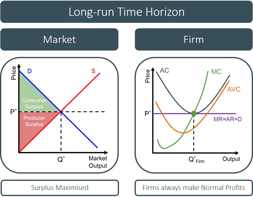
This outcome is the most efficient market equilibrium that can be achieved because of the fact that there is no deadweight loss triangle present unlike in other market structures e.g. a monopoly. 

It creates the most efficient outcome because firms that operate in a perfectly competitive market are classed as productively efficient in the long-run as they end up making normal profits and producing at the minimum of the average cost curve. 

Also most firms can be classed as allocatively efficient in the long-run as firms produce at the point where P=MC. However, this only holds if firms are producing in a market with no externalities present. This is because when there are externalities present, private costs and benefits do not equate to social costs and benefits. If the marginal social benefit and costs do not equate then this means that consumer and producer surplus cannot be maximised and this means there must be a better allocation of resources available in the market.

However, despite perfect competition providing efficient results, one type of efficiency that is not achieved is dynamic efficiency. This is because in order for firms to be incentivised to achieve dynamic efficiency they need to make supernormal profit to enable them to undertake the investment required for the research and development needed to innovate the production process. It is unlikely that this will be achieved in perfect competition because the assumption of perfect knowledge across all firms means that firms can just replicate any new products or new techniques developed in the production process, removing any competitive/cost advantage this type of investment is meant to develop. Also the fact that firms cannot make supernormal profit in the long run means that they will never be in a position to be able to protect the advantages of their investment and will not be encourage to make the changes required. The fact that dynamic efficiency is not achieved creates wider implications for the economy because it is investment that drives the long-run trend growth rate and therefore if investment is stunted because of this form of competition, long-run growth will be permanently revised at a lower level. 

The final point to mention regarding perfect competition is the theoretical model can be used as a yardstick to compare other market structures against. This is because in reality industries are never really perfectly competitive, but by relaxing some of the assumptions of perfect competition it may mirror some types of market structures (e.g. monopolistic competition) and therefore allow us to asses and evaluate those markets. For instance, the closer an industry is to perfect competition, the closer it is to the efficiency results which fosters improved services and products. 

When buyers and sellers have complete information concerning factors that could influence decisions to buy and how to produce a good i.e. prices and quantities for sale, how to make the goods and the most efficient production techniques.

Below is a graphic to highlight the main factors that have to hold for agents to have full and complete information about the market.

When buyers and sellers have complete knowledge concerning factors that could influence decisions to buy and how to produce a good i.e. prices and quantities for sale, how to make the goods and the most efficient production techniques.

Is a term used to relate to goods that have a price elasticity of demand value of infinity. This essentially means that the quantity demanded by consumers for these types of goods depends severely on the market price i.e. if the price increases or decreases this will cause demand to collapse to zero for this good. This is normally a result of their being a large number of perfect substitutes available in the market. 

We can represent a good that has a perfectly elastic demand curve as a demand curve that is horizontal at the market price. This is shown below:

Any amount of a good can be demanded at or below the price level contained in the demand curve while there will be no demand for the good at a higher price. As demand cannot be determined the price elasticity of demand is infinite. Price elasticity of demand is also infinite at the point where demand is zero.

Refers to goods that have a price elasticity of supply value equal to infinity. This essentially means that any amount of a good will be supplied at the prevailing price, but nothing is supplied below this prevailing price. 

This is shown in the diagram below:

So in this case if the price falls to P2 (even with a small price fall) the quantity supplied by the firm will instantly drop to zero. This is normally a theoretical application of PES to supply curves.

Is a term used to relate to a good that has a price elasticity of demand value of 0. This essentially means that the quantity demanded by consumers for this good does not depend on the price of the good i.e. consumers will demand the same quantity of the good at every possible price.

We can represent a perfectly inelastic demand curve via a vertical demand curve as shown below:

For this demand curve the PED values are equal to 0 at all points and therefore changes to prices have no effect on quantity demanded e.g. diabetic patients demand for insulin.

Perfectly inelastic demand also arises if the price of a good is zero and quantity demanded is at its maximum possible level. However, this is only of theoretical significance as even a 1p rise in price will mean that elasticity rises above this level.

This refers to when only one quantity of a good can be supplied at any given price. As a result this means the price elasticity of supply (PES) value is equal to 0.

The shape of a perfectly inelastic supply curve is shown below:

The supply curve is vertical at the specific quantity supplied of Qs. This curve highlights that any change in price does not cause a change in the quantity supplied. It is very rare for firms to face an inelastic supply curve as traditionally firms will always supply more when the price of the good they are supplying increases. An example of this might be the UK property market as demand has been outstripping demand, forcing house prices up. This is particularly the case in areas such as London where it is almost impossible to find new land to build properties. Which is an explanation over why house prices are so much expensive in this area. 

The amount of income a household could spend over its lifetime without reducing the value of its assets e.g. dividends on shares or interest on deposits.

The Phillips Curve is an economic model that illustrates a stable inverse relationship between the inflation rate and the unemployment rate. It is used to show policymakers that there is an exploitable trade-off between the unemployment rate and the inflation rate i.e. unemployment can be reduced at the expense of higher inflation.

The Phillips Curve was first established in 1958 by an economist named A. W. Phillips, in which 96 years worth of data was collected on wage inflation and unemployment. The data points were plotted on a graph, with the unemployment rate on the x axis and the wage inflation rate on the y axis. A line of best fit was then drawn through this collection of data points and this line of best fit was downward sloping, showing the inverse relationship between the two variables and this has now become known as the Phillips Curve.

Since then the Phillips Curve has been adapted to provide more theoretical importance for policymakers to consider when setting economic policies. As now the inflation rate (price inflation) is used instead of wage inflation. The result of the inverse relationship still holds but now concerns the inflation rate instead. 

Below is a diagram to illustrate the basic convex shape of the conventional Phillips curve discovered by A. W. Phillips. This curve illustrates the main policy trade-off facing governments i.e. a government cannot achieve both low unemployment and inflation. 

 

By using this curve the government can aim to reduce the unemployment rate by introducing an aggregate demand stimulus, which increases real output and unemployment in the process, but at the same time this creates inflationary pressures (demand pull inflation) as a result of a positive output gap emerging. This positive AD shift can be represented by a movement up the Phillips curve to signify an increasing inflation rate when the unemployment rate decreases.

 

However, in the 1970's the smooth, stable inverse relationship seen in the Phillips curve between the inflation rate and the unemployment rate began to break down as suddenly data points were being recorded where both the unemployment and inflation rate were high and this contradicted the main result of the original Phillips curve. 

As a result of this, it was commonly accepted that in the long-run the Phillips curve would take a different form and the trade-off between inflation and unemployment would disappear. The long run Phillips curve is vertical at the natural rate of unemployment and depicts no exploitable trade-off between the inflation rate and the unemployment rate. The key difference for policymakers when dealing with the LRPC is that demand side policies designed to reduce the unemployment rate below the natural rate do not prove effective as workers re-adjust their wage aspirations in light of higher inflation, which means unemployment  always remains at the same level in the long-run but with higher inflationary pressures. So effectively the long run Phillips curve is established by multiple shifts of the short run Phillips curve

The distinction between the shape of the short run and long run Phillips curve is shown below.

 

Therefore, in the long-run the only way to reduce the natural rate of unemployment is to introduce specific supply side policies which aim to improve the productive capacity of the economy by creating sustainable unemployment reductions, which create an LRAS shift (outwards) in the process. Persistent demand side policies will create an inflationary outcome for the economy. However, these policies must be specifically targeted to improve worker flexibility otherwise will not create the curve movements required to reduce unemployment below the natural rate.

The Phillips curve is a contentious issue as it all depends on your political persuasion, in terms of how the curve is interpreted. But, the main evaluation points regarding the Phillips curve are:

• Recent evidence from the UK economy appears to contradict the main theoretical result of the Phillips Curve i.e. data points reflecting high unemployment and inflation rate.
• The current version of the Phillips Curve is an adapted version of the original i.e. shows price inflation instead of wage inflation.
• The Phillips Curve may be subject to measurement errors/biases because data quality and changing nature of data will affect the outcome depicted by the Phillips curve.
• The distinction between the short run and long run Phillips Curve i.e the trade-off is not present in the long-run.
• To take into account the type of expectations that economic agents have i.e. if economic agents have rational expectations it might mean there is no short-run and long-run distinction between the Phillips Curve. 

The level of output that firms plan to supply. This can be problematic as decisions have to be taken before actual demand conditions are known. This is particularly problematic in agriculture when supply decisions have to be made many months in advance.