Economic Terms

Describes a firm that is already in position in the market. In a contestable market incumbent firms are unable to enjoy abnormal profits due to hit-and-run entry.

 

A way of simplifying the measurement of averages (e.g. inflation and stock markets) and comparing different data series by establishing a base of 100.

Index numbers are calculated by selecting a base year and then dividing each of the values by that base year value and seeing the proportionate change relative to the base year rather than the percentage change. It is important to remember that index numbers DO NOT show the percentage change in a variable over time. The main benefit of index numbers is they allow cross-variable comparisons with variables that use different measurements. The table shows how the index numbers for GDP are calculated using the method mentioned above.

 

Taxes that are imposed on transactions. e.g. VAT, fuel duty, insurance premium tax.

Taxes that are imposed on transactions. e.g. VAT, fuel duty, insurance premium tax.

Taxes that are imposed on transactions. e.g. VAT, fuel duty, insurance premium tax.

The demand for a good/service from an individual consumer or firm.

This is a technical economy of scale. Many economies of scale can only be captured by using large items of equipment that must be continuously used to full capacity. This means that smaller suppliers can’t access the same economies of scale if the equipment isn’t available on a smaller scale.

When the percentage change in demand is less than the percentage change in price. In this case the PED elasticity value will lie between 0 and -1.

To identify the shape of an inelastic linear demand curve we do not focus on the gradient of the curve as this does not actually determine elasticity. Crucially, it is the position of the demand curve that determines elasticity. This is because all linear demand curves contain portions on the curve which can be classed as elastic, inelastic and unit elastic. Any demand curve shown (like the one below) is just a section of a much larger demand curve that extends beyond the axis.

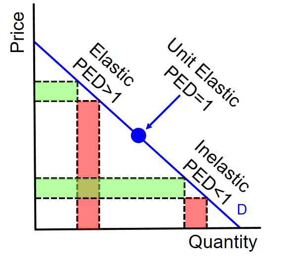
So effectively we can see that the midpoint of the demand curve is when unitary elasticity is achieved. The bottom half of the curve is inelastic, because if the price rises - at any point below the midpoint - expenditure increases despite a quantity fall. The top half of the curve is elastic, because if the prices rises - at any point above the midpoint - expenditure decreases due to a large quantity fall.

Therefore, the easiest way to determine an inelastic demand curve is to extend the section of the demand curve drawn and identify which axis it intersects. If the demand curve intersects the x axis we can judge it as being an inelastic demand curve as we must be focusing on the bottom of the demand curve. An example of an inelastic demand curve is shown below.

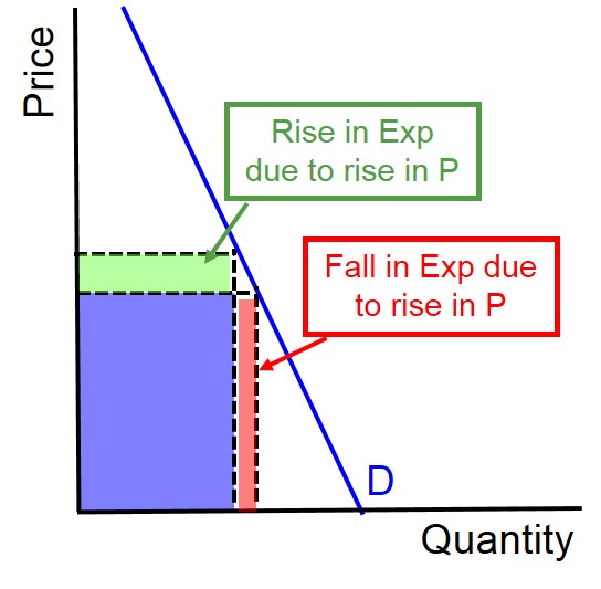
This diagram highlights the changes in expenditure for a producer that occurs when there is a small price rise in a market with inelastic demand. When a demand curve is relatively inelastic, it means that consumers are price insensitive to changes. In this instance, a price rise leads to a small fall in demand as consumers refuse to switch to alternative cheaper substitutes. 

When the proportionate change in supply is less than the proportionate change in price. In this case the PES elasticity value will be below 1.

Below is an example of an inelastic supply curve:

The supply curve has the typical upward sloping relationship between price and quantity supplied because the profit incentives that firms face are greater when the price increases. However, with an inelastic supply curve firms ability to raise output in line with a price increase is restricted due to a number of different factors. Which is the main reason why with this type of supply curve the change in the quantity supplied is proportionately less than the price.

These factors are:

1. Amount of Spare Capacity - If a firm has very little spare capacity left, they will not have the sufficient resources to increase output when the price rises.

2. Length of Production Process - If a firm is producing a good that has a long production process their ability to respond to price increases by raising output is restricted as they are unable to raise supply within a short period of time. This is often the case in agricultural markets.

3. Factor Substitutability - A firm will always wish to produce the good that has the highest price, as this is the good that will yield the highest level of profit. However, if firms are unable to transfer their factors of production towards different production processes, this ability to increase output in line with prices is restricted.

A type of good where demand for the good decreases as INCOME rises e.g. own value brand products.

Below is a diagram to illustrate the basic demand curve structure for an inferior good. If the level of real income increases this causes an inward shift of the demand curve as consumers disposable income increases they switch to better quality products that they derive a greater level of utility from. Vice versa if the level of real income decreases this causes an outward shift of the demand curve as consumers can no longer afford normal goods and therefore they switch to cheaper alternatives which are of inferior quality.